A guide to RWKV V3

Introduction

RWKV is an alternative to the transformer architecture. It's open source and has it's own paper over here. I found out about it sometime back in a paper club and thought i'd write a short article about it with what I had learnt.

Here are some other resources which you might find useful about RWKVs

RKWV by Picocreator This is a markdown file that was used by one of the contributors - Picocreator to give a short presentation on the RWKV architecture.
RKWV in 100 lines Which covers the implementation of RWKV in 100 lines of code. Much of this article is based off the content here - I try to extend and provide my own intuition for some proofs. I've also attached a colab notebook for you if you want to play with the code.

With that being said, let's dive into RWKVs.

I'm using the 430M model here. Hence why my embedding space is 1024. Other models might differ so do take note if you are experimenting with the larger models.
Do note that there are some issues with numerical instability in the simplified version provided by johanwind which have been fixed in the implementation in Blink's repo. This is not production code.

Background

Transformers

For a better and more thorough explanation, do check out GPT in 60 Lines of numpy by Jay K mody. Some of the content here is paraphrased and I suggest going to the source for the best understanding.

What is a transformer? Normally today, when we talk about transformers, we're refering to GPTs - Generative Pre-Trained Transformers. These are huge models that have billions of parameters and are trained on lots of data. This enables them to be able to have an underlying understanding of language.

How do they do this? You can think of a transformer as having the following function signature where

n_seq: This is the size of the initial data passed in. It has to be less than or equal to the context length.
n_vocab: Our transformer outputs a prob distribution for each character in the input + the new predicted output.

def gpt(inputs: list[int]) -> list[list[float]]: # inputs has shape [n_seq]
# output has shape [n_seq, n_vocab]
	output = # beep boop neural network magic
	return output

A big part of this magic happens because of the self-attention mechanism, which gives transformers their special powers but also increases the time needed to make a prediction.

Attention and Why it sucks

Some parts of this explanation are from Code Emporium's Excellent explanation on Transformers which you can view here

The most important to take away from this section is that Attention scales quadratically. That's the single biggest bottleneck when we want to scale transformers to do more things.

Let's see a graphical representation of what that might look like

A few things here to point out

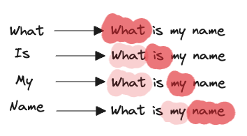
Each word never sees a word that's beyond it's position. In the context of GPT when we are doing next token prediction, we don't the model to "see the future"
Every single word prior to a word is compared against it to determine its relevancy to predicting the next word.

In our example above,

What is compared to What (1 comparison )
Is is compared to What and Is ( 2 comparisons )
My is compared to What,Is and My ( 3 comparisons )
Name is compared to What, Is, My and Name ( 4 comparisons )

In some cases, (1) might not hold (Eg. in Translation) where grammar structures differ between languages but for a GPT, this is normally the case.

because (2) is happening, then this means that the number of comparisons for a string that has been broken down into n tokens is going to be

1 + 2 + \dots + n = \frac{n(n+1)}{2}

which is quadratic in nature. This is an oversimplification of attention but you get the idea. That's why it gets more and more costly as we expand our models context sizes because there are simply more comparisons to be made.

We cannot cache these previous lookups in a transformer. This is one of the biggest problems with Transformers that RWKV doesn't have as you'll see down below.

In transformers, the self-attention mechanism computes query, key, and value vectors for each word in the input sequence and uses the dot product of these vectors to determine the attention scores. This process is sensitive to the specific tokens in the input sequence, and as a result, caching the attention scores for one sequence may not be applicable to a subsequent sequence.

RWKV

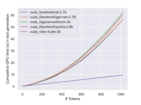
RWKVs aim to solve the issue of attention by approximating attention with a linear operation instead. This results in 1-1.5x cheaper training costs and around 10x cheaper inference costs, especially as the number of tokens passed into the model increase over time.

We can see this with the following graphic from the RWKV paper that shows how the inference cost grows with respect to the token count. This means that as the length of what we pass in increases, we enjoy significantly lower inference time with the RWKV architecture.

High Level Understanding

RWKVs operate using two main mechanisms

A world state : This stores information on information such as previous computations
Temporal mechanism : RWKV uses a decay function to reduce the weightage of past information w.r.t new information.

However, as a result of a world state, the RWKV model has a major weakness - it might end up discarding content which is relevant but not explictly requested at the start of the prompt.

As a result, when we're prompting the RWKV model, we want to use the following syntax

{{INSTRUCTION}}

{{CONTEXT}}

{{ANSWER}}

instead of the typical format of

{{CONTEXT}}

{{INSTRUCTION}}

{{ANSWER}}

Architecture

Sigmoid

Intuitively, the sigmoid function is used as a activation function in both the time-mixing and acts as a forget gate in our Time Mixing and Channel Mixing blocks. Since all values are effectively coerced from 0 to 1, A value closer to 0 means the information should be forgotten, while a value closer to 1 means the information should be retained.

This plays a crucial role in determining the relevance of information from prior steps, allowing the network to selectively retain or discard information based on the current input and previous hidden state

State

In essence, we can think of the state as being comprised of the following components

[layerState,layerState,.... ]

Inside each layerState, we have a total of 4 subarrays

state = np.zeros((N_LAYER, 4, N_EMBD), dtype=np.float32)

inside the state, we allocate space for each element as

0 : prevX computation
1 : prevNum Computation
2 : prevDen Computation
3 : prevChannelMixing result

This helps our model to be able to get some concept of time. Note that (3) is mostly used to replace the short-term memory ( since it can only look back a single step )

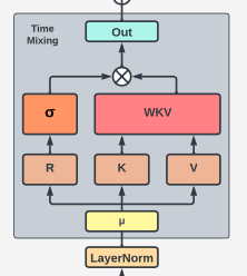
Time-Mixing

Time mixing approximates attention and can be likened to the LSTM component of a traditional RNN architecture. This is because it has access to two things

Previous World State
Learned weights to determine how to combine previous computations and new computations.

Intuitively as time t increases, then the vector is dependent on a long history and a summation of an increasing number of terms. This creates a memory which can keep track of information provided in an earlier context.

We can visualise the entire architecture of the time-mixing block as seen below.

Let's look at a function to compute time-mixing

# Time mix layer with the various params
def time_mixing(
		# Incoming state of the current token
		x,
		# Previous token shift state
		last_x,
		# Previous state, split across 2 values to prevent overflows
		last_num, last_den,
		# Various weights, all trainable
		decay, bonus, mix_k, mix_v, mix_r, Wk, Wv, Wr, Wout
	):

	# Given the incoming state, and the previous token shift state
	# compute R,K,V values. The `x * mix + last * (1-mix)` pattern
	# helps the model have trained weights to decide which factors
	# it wants to use for the respective process
    k = Wk @ ( x * mix_k + last_x * (1 - mix_k) )
    v = Wv @ ( x * mix_v + last_x * (1 - mix_v) )

	# Since R is used for the final gating of output (similar to attention score)
	# you can view this as a lite form of Q @ K
    r = Wr @ ( x * mix_r + last_x * (1 - mix_r) )

	# Here we effectively do magic(last_state + k) * v
	#
	# But in essence, its the "summation with decay" of all the past expotents
	# divided by another set of expotents for numeric stability
	# (aka anti exploding gradients).
	#
	# Bonus is used to boost the signal for the WKV value
    wkv = (last_num + exp(bonus + k) * v) / \
          (last_den + exp(bonus + k))

	# We compute the cumulative sum, for the next round, where it
	# is stored and forwarded as a state, with a gradual
	# decay value on the previous value.
	#
	# `exp(-exp(decay))` is essentialy a math hack to ensure decay
	# is between 0-1, and will gradually fade out past value if desired
	#
	# `exp(k) / exp(k) * v` is the summation accumulation of the current state
	# to be used in the next time mix
    num = exp(-exp(decay)) * last_num + exp(k) * v
    den = exp(-exp(decay)) * last_den + exp(k)

	# sigmoid then acts looseley as both a part of Q in QKV,
	# and as a forget gate in LSTM (together with decay)
	# for the WKV values
    rwkv = sigmoid(r) * wkv

	# And finally that gets normalized into an output, and next state
    return Wout @ rwkv, (x,num,den)

This function implements the following equations of

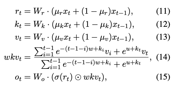
In our function, We have the parameters of

last_x,last_num, last_den : These are all stored in a huge (N_Layers, 4,N_embeddings) array and simply store the previous computations for each layer.
- last_x: $x_{t-1}$
- last_num: $wkv_{t-1}$ numerator
- last_den: $wkv_{t-1}$ denominator
decay, bonus, mix_k, mix_v, mix_r, Wk, Wv, Wr, Wout
- decay : w parameter can be treated as $e^{-\text{decay}}$
- bonus : This is equivalent to the u parameter above
- mix_k,mix_r and mix_v are equal to $\mu_k,\mu_r,\mu_t$
- Wk,Wv,Wr and wout are equivalent to W_k,W_v,W_r and W_o above
Note here that $\sigma$ simply represents the sigmoid activation function.

In the code above, it might be a little bit difficult to visualise the dimensions so

(1024,1024) : $W_r, W_k, W_v$
(1024, ): $\mu_r,x_t,x_{t-1},\mu_k,\mu_v$ , decay, bonus

This means that essentially

r_t,k_t

and

v_t

are all going to be of the dimension (1024,) and the final output of this function will be of (1024,).

What's interesting about this is that information on all previous tokens seen is stored in a 1024 dimensional array. Compare this to transformers that generate a n_seq x n_embd array due to the attention mechanism. Is attention truly even needed?

Inductive Proof

I was slightly confused by these 4 lines of code since I couldn't quite understand the leap from last_num to num and den to last_den.

wkv = (last_num + exp(bonus + k) * v) /      \
          (last_den + exp(bonus + k))
rwkv = sigmoid(r) * wkv

num = exp(-exp(decay)) * last_num + exp(k) * v
den = exp(-exp(decay)) * last_den + exp(k)

Which tries to implement the step of

wkv_t=\frac{\sum_{i=1}^{t-1}e^{-(t-1-i)w+k_i}v_{i} + e^{\mu+k_t}v_t}{\sum_{i=1}^{t-1}e^{-(t-1-i)w+k_i} + e^{\mu+k_t}}

Let's try to build the intuition for this step by step. Let's say we wanted to take the sum of all the elements in the following sum. ( This is present in the numerator ).

\sum_{i=1}^{t-1}e^{-(t-1-i)w+k_i}v_{i}

Let's also designate the sum of all the elements defined in the sum as

\alpha_{t-1}

where we are summing elements from 1 to

t-1

. How do we get from

\alpha_{t-1}

\alpha_{t}

? If we look at the term

\alpha_{t-1}

, we can see that the final value of the summation is going to be

e^{-(t-1-(t-1))w+k_i} = e^{k_{t-i}}

Well, what about the second last value of the summation then? it's going to be

e^{-(t-1-(t-2))w+k_{t-2}} = e^{-w + k_{t-i}}

This means that we can therefore link

\alpha_{t-1}

with

\alpha_{t}

by doing

\sum_{i=1}^{t-1}e^{-(t-1-i)w+k_i}v_{i} = \sum_{i=1}^{t-2}e^{-(t-1-i)w+k_i}v_{i} + e^{k_{t-1}}

We can perform a similar substituition to get

\beta_{t} =\beta_{t-1}+ e^{k_{t-1}}

num = exp(-exp(decay)) * last_num + exp(k) * v
den = exp(-exp(decay)) * last_den + exp(k)

We can then rewrite our equation for

wkv_t

wkv_{t} = \frac{\alpha_{t-1} + e^{\text{bonus} + k_{t}}v_t }{\beta_{t-1} + e^{\text{bonus} + k_{t}}}

which corresponds to our implementation of

wkv = (last_num + exp(bonus + k) * v) /      \
          (last_den + exp(bonus + k))
    rwkv = sigmoid(r) * wkv

Channel Mixing

The channel mixing is the short term component of the system - it only has access to the previous value and it takes a weighted sum of the previous and current value that it has calculated.

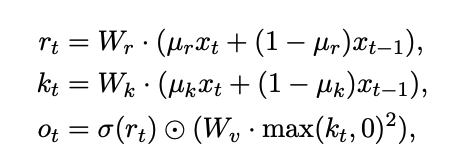It's significantly easier to understand. Note that all these parameters are learned parameters with the exception of the $x_{t-1}$ values.

Our channel mixing function is implemented as

def channel_mixing(x, last_x, mix_k, mix_r, Wk, Wr, Wv):
    k = Wk @ ( x * mix_k + last_x * (1 - mix_k) )
    r = Wr @ ( x * mix_r + last_x * (1 - mix_r) )
    vk = Wv @ np.maximum(k, 0)**2
    return sigmoid(r) * vk, x

It's interesting here to note that
- $w_k$ has a dimensionality of $[4096,1024]$
- $w_v$ has a dimensionality of $[1024,4096]$

This means that we perform a scaling in the channel_mixing step from an initial dimensionality of 1024 to a dimensionality of 4096. This is very similar to the feed forward network that is used as a transformer.

Bringing it together

If we look at the code for RWKV in 100 lines, we notice that the RWKV architecture for the 400M model comprises 24 layers of the same block.

Each block comprises

1 initial layer norm ( Constant work since the size of the input is fixed as a (1024,) matrix )
1 time_mixing step
1 layer norm ( Also fixed size input of (1024,) )
1 channel mixing step

All of the operations that we perform in the time_mixing and channel_mixing step are all going to linearly scale with the size of our context.

The way I understand it is that since information on all previous token is compressed into a single token value

Time Mixing requires a constant number of operations per prediction step
Channel Mixing also requires a constant number of operations per prediction step

Therefore, for every additional token we want to predict or want to add into our context, we have a constant amount of work to be done for each of these tokens. Therefore, this means that the amount of computational work we need to perform will scale roughly linearly with the amount of tokens we eventually need to predict/proccess.